Score
The next step is to examine the forecast skill. This is done by comparing the actual trajectories to the forecasted trajectories. We will see different patterns in the forecast skill depending on whether the system is dominated by deterministic or noisy dynamics.
Regression
For regression, there are two ways to measure the accuracy of the results. The default score method is the coefficient of determination. This is the default for many of scikit-learn’s scoring functions as well. Additionally, the correlation coefficient can also be used to score a continuous variable.
These can be called by:
score1 = M.score(ytest, how='score') # Coefficient of determination
score2 = M.score(ytest, how='coeff') # Correlation coefficient
Coefficient is useful when you are interested in making precise forecasts and correlation coefficient is useful when you are interested in accurate forecasts. For example, consider the following plot where blue are the actual values and green are the predicted values.
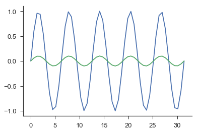
The correlation coefficient for these predictions would be equal to one, while the coefficient of determination would be 0.19. Depending on on your interest, either statistic could be useful.
Classification
For classification, there are two ways to measure prediction skill. The first is by a simple percent accuracy. This calculates what percent were correctly predicted. The second way is by klecka’s tau which attempts to normalize by the distribution of classes.
score1 = M.score(ytest, how='compare') # Percent correct
score2 = M.score(ytest, how='tau') # Kleck's tau
Percent correct is useful when you have balanced classes, but not useful when the classes are skewed. For example, if there are two classes and class 1 makes up 95% of the data. Predicting a 1 everywhere would show you 95% accuracy while klecka’s tau would show an accuracy of about -8.8. Again, both stastics could be useful in the correct context.
Distinguishing Determinism
Here we analyze the logistic map with varying levels of noise as indicated by the title.
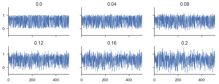
To begin, we follow the fit, predict_individual, and score routine as usual for every time series. Interested readers can find the code in the jupyter notebook. Next we look at the correlation coefficient for each series for one prediction forward in time. The legend refers to the level of noise that was added to the time series.
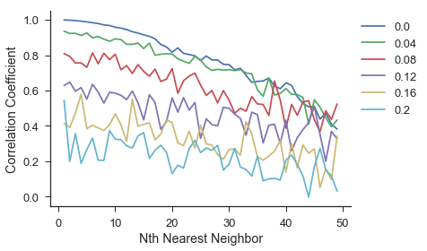
Analyzing the plot above, we can see that as the amount of noise increases, the forecast skill decreases. This is to be expected as adding stochasticity to a system makes it inherently more difficult to forecast. The next thing to notice is that the forecast skill decreases more rapidly for the series with less noise. It is more important in deterministic systems to grab neighbors that are nearby in space.