Quick Example

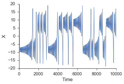
To illustrate the utility of this package we will work with the Lorenz system. The Lorenz system takes the form of :

\[ \begin{align}\begin{aligned}\frac{dx}{dt} = \sigma (y - x)\\\frac{dy}{dt} = x(\rho - z) - y\\\frac{dz}{dt} = xy - \beta z\end{aligned}\end{align} \]

After numerically solving this system of equations, we are going to make forecasts of the \(x\) time series. Note that this series, while completely deterministic (there is no randomness associated with any of the above equations), is a classic chaotic system. Chaotic systems are notoriously difficult to forecast (e.g. weather) due to their sensitive dependance on initial conditions and corresponding positive Lyapunov exponents.

There is a function in skedm.data that numerically solves the lorenz system using scipy’s built in integrator with a step size of 0.1 seconds. For example:

import skedm.data as data

X = data.lorenz(sz=10000)[:,0] #only going to use the x values from the lorenz system

In attempting to use the \(x\) time series to reconstruct the state space behavior of the complete lorenz system, a lag is needed to form the embedding vector. This lag is most commonly found from the first minimum in the mutual information between the time series and a shifted version of itself. The first minimum in the mutual information can be thought of as jumping far enough away in the time series that new information is gained. A more inituitive but less commonly used procedure to finding the lag is using the first minimum in the autocorrelation. The mutual information calculation can be done using the embed class provided by skedm.

import skedm as edm

E = edm.Embed(X) #initiate the class

max_lag = 100
mi = E.mutual_information(max_lag)

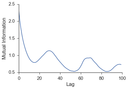
The first minimum of the mutual information is at \(n=15\). This is the lag that will be used to rebuild a shadow manifold. This is done by the embed_vectors_1d method. A longer discussion about embedding dimension (how the value for embed is chosen) is found in the Embed section.

lag = 15
embed = 3
predict = 30 #predicting out to double to lag
X,y = E.embed_vectors_1d(lag,embed,predict)

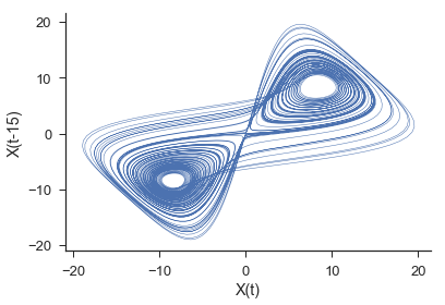
The plot above is showing only X[:,0] and X[:,1]. The full three dimensional embedding preserves the geometric features of the original lorenz attractor.

Now that we have embed the time series, we can use trajectories in the state space near a point in question to generate forecasts of system behavior and see if the system contains the hallmarks of nonlinearity, namely high forecast skill when using local neighbor trajectories in the reconstructed space. First we split the data into a training set and testing set. Additionally, we will initiate the Regression class.

#split it into training and testing sets
train_len = int(.75*len(X))
Xtrain = X[0:train_len]
ytrain = y[0:train_len]
Xtest = X[train_len:]
ytest = y[train_len:]

weights = 'distance' #use a distance weighting for the near neighbors
M = edm.Regression(weights) # initiate the nonlinear forecasting class

Next, we need to fit the training data (rebuild the shadow manifold) and make predictions for the test set (22 seconds on a macbook air).

M.fit(Xtrain, ytrain) #fit the data (rebuilding the attractor)

nn_list = [10, 100, 500, 1000]
ypred = M.predict(Xtest,nn_list)

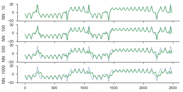
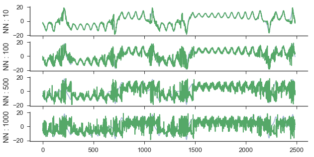
ypred is a list of 2d arrays that is the same length as nn_list. Each 2d array is of shape (len(Xtest), predict). For example, the second item in ypred is the predictions made by taking a weighted average of the closest 100 neighbor’s trajectories. We can view the predictions using 10, 100, 500, and 1000 neighbors at a forecast distance of 30 by doing the following:

fig,axes = plt.subplots(4,figsize=(10,5),sharex=True,sharey=True)
ax = axes.ravel()

ax[0].plot(ytest[:,29],alpha=.5)
ax[0].plot(ypred[0][:,29])
ax[0].set_ylabel('NN : ' + str(nn_list[0]))

ax[1].plot(ytest[:,29],alpha=.5)
ax[1].plot(ypred[1][:,29])
ax[1].set_ylabel('NN : ' + str(nn_list[1]))

ax[2].plot(ytest[:,29],alpha=.5)
ax[2].plot(ypred[2][:,29])
ax[2].set_ylabel('NN : ' + str(nn_list[2]))


ax[3].plot(ytest[:,29],alpha=.5)
ax[3].plot(ypred[3][:,29])
ax[3].set_ylabel('NN : ' + str(nn_list[3]))

sns.despine()

The next step is to evaluate the predictions with the score method. The score method defaults to using the coefficient of determination between the actual values and predicted values.

scores = M.score(ytest) #score

fig,ax = plt.subplots()

for i in range(4):
    label = 'NN: ' + str(nn_list[i])
    ax.plot(range(1,31),scores[i],label=label)

plt.legend(loc='lower left')
ax.set_ylabel('Coefficient of Determination')
ax.set_xlabel('Forecast Distance')
ax.set_xlim(1,30)
sns.despine()

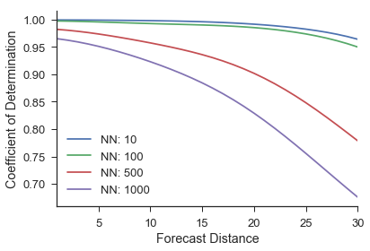
scores has shape (len(nn_list),predictions). So this example will have a shape that is (4, 30). For example, the first spot in the score array will be the coefficient of determination between the actual values one time step ahead and the predicted values one time step ahead using 10 near neighbors. As expected, the forecast accuracy decreases as more near neighbor trajectories are averaged together to make a prediction and as we increase the forecast distance.

Additionally, instead of averaging near neighbor trajectories, it is possible to look at the forecast of each neighbor individually. This is done by simply calling the predict_individual method as below.

ypred = M.predict_individual(Xtest,nn_list)

Then again, we can calculate the score and visualize it as:

score = M.score(ytest)
fig,ax = plt.subplots()

for i in range(4):
    label = 'NN: ' + str(nn_list[i])
    ax.plot(range(1,31),score[i],label=label)

plt.legend(loc='lower left')
sns.despine()
ax.set_ylabel('Coefficient of Determination')
ax.set_xlabel('Forecast Distance')
ax.set_xlim(1,36);

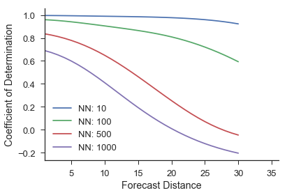
As we can see, by not averaging the near neighbors, the forecast skill decreases and the actual forecast made becomes quite noisy. This is because we are now using single trajectories that are not nearby in the reconstructed space to make predictions. This should intuitively do worse than picking nearby regions.