Predict

At the heart of this software package for emperical dynamic modeling is the k-nearest neighbors algorithm. In fact, the package uses scikit-learn’s nearest neighbor implementation for efficient calculation of distances and to retrieve the indices of the nearest neighbors. It is a good idea to understand the k-nearest neighbor algorithm before interpreting what this package implements.

For the regression case, we will look at a zoomed in version of trajectories from the lorenz system projected in two-dimenisonal space. The red dots are the actual points that make up the trajectory depicted by the blue line and the green box is the point that we want to forecast. The trajectory is clockwise.

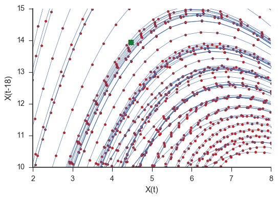
In this section of the Lorenz attractor, we can see that the red points closest to the green box all follow the same trajectory. If we wanted to forecast this green box, we could grab the closest red point and see where that ends up. We would then say that this is where the green box will end up.

Grabbing more points, however, might prove to be useful since our box lies between a couple of the points. It might be better to average the trajectories of, for example, the three nearest points to make a forecast.

For this case, grabbing more and more near neighbor trajectory points will be detrimental to the forecast as those far away points are providing information from regions of the space that are not useful for projecting the local dynamics of our test, green point.

It is illustrative to see the effects of adding noise to this system as shown in the plot below.

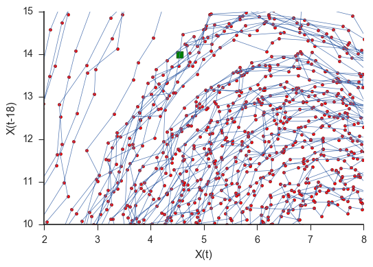
To the extent that noise becomes dominant relative to the local space dynamics, the gain from using only local trajectories goes away and predictability levels off or increases as one grabs more and more neighbor trajectories.