Performance

Here we provide some basic guidelines on performance. All of these were run on an early 2015 macbook air. The code can be found in the accompanying jupyter notebook.

As a baseline, the example given in the Quick Example section completes in 4.2 seconds.

X = data.lorenz(sz=10000)[:,0] #only going to use the x values
E = edm.Embed(X)

lag = 15
embed = 3
predict = 30 #predicting out to double to lag
X,y = E.embed_vectors_1d(lag,embed,predict)

train_len = int(.75*len(X))
Xtrain = X[0:train_len]
ytrain = y[0:train_len]
Xtest = X[train_len:]
ytest = y[train_len:]

M = edm.Regression() # initiate the nonlinear forecasting class
M.fit(Xtrain,ytrain) #fit the training data

nn_list = [10,100,500,1000]
ypred = M.predict(Xtest,nn_list)
score = M.score(ytest) #score the predictions against the actual values

In the following sections we expand this example by changing the amount of near neighbors, training size, and testing size. This will give us an idea of the performance impacts of exploring different data sets.

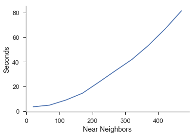
Near Neighbor

Here we increase the amount of near neighbors with everything else held constant. This is the time it takes to complete every near neighbor value between the one given on the x axis and 1. For example, the first point is the amount of time it takes to complete the near neighbor calculation for [1,2,3,4,5,6,7,8,9,10] near neighbors.

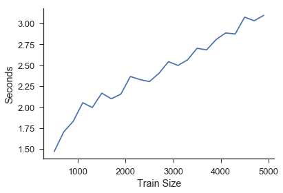
Train Size

Here the testing size, and the number of near neighbors is held constant. We simply iterate through the length of the training set.

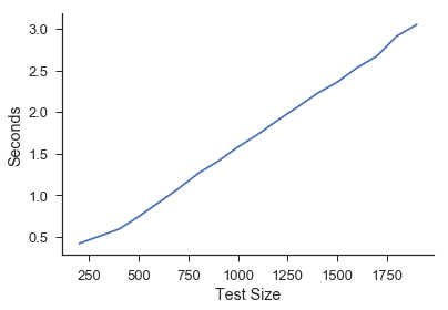
Test Size

Here the training size and the number of near neighbors is held constant. We simply iterate through the length of the testing set.